
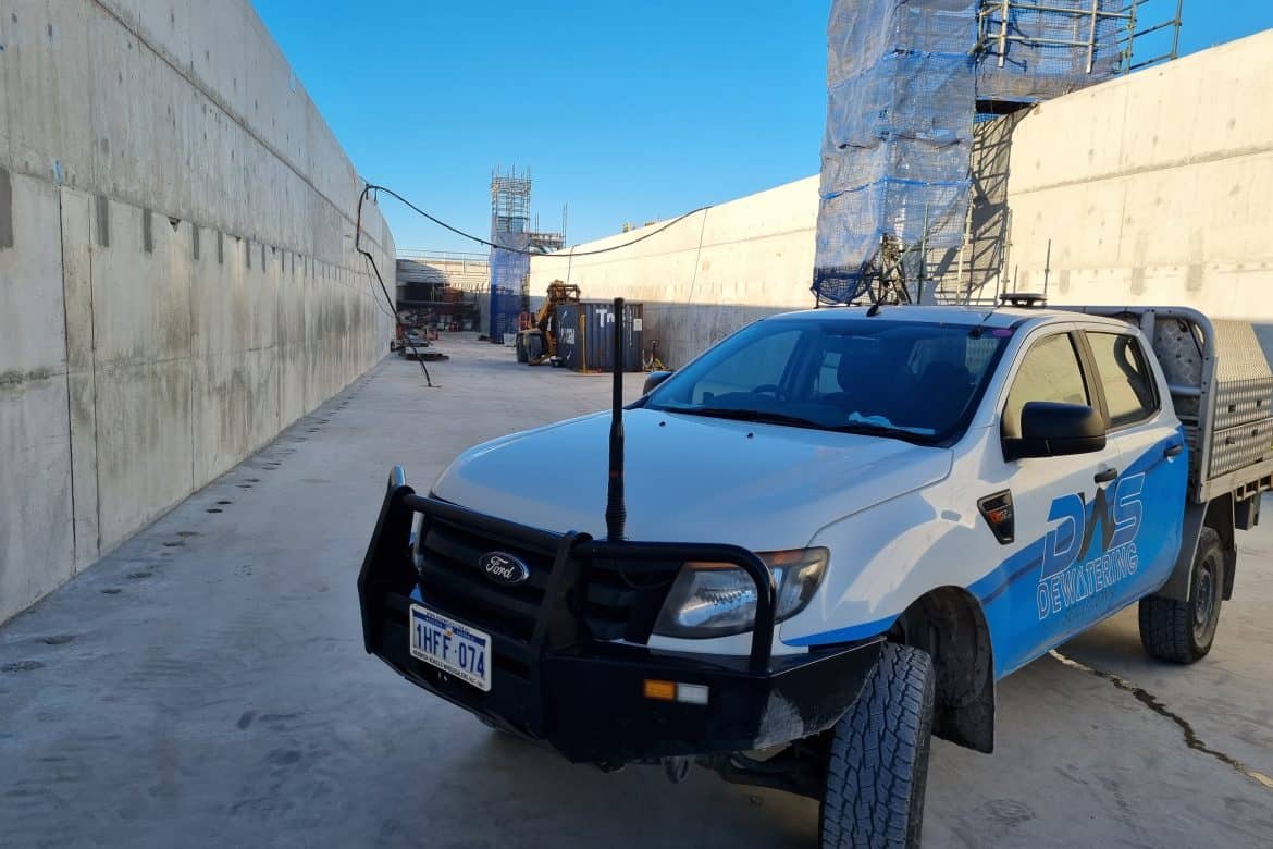
An excavation can appear dry at the surface while groundwater pressure below the formation level is still capable of lifting, softening or destabilising the base. A sound deep well dewatering calculation is therefore not simply a pump-sizing exercise. It is the basis for deciding whether a proposed system can achieve the required drawdown, maintain stable ground conditions and keep the programme moving without creating off-site or environmental issues.
For major civil, construction and mining works, the calculation must translate ground investigation data into a practical field system: well depth, screen interval, pump duty, well spacing, discharge arrangements and monitoring requirements. It also needs enough contingency to deal with the conditions that boreholes and models do not fully reveal.
Start with the groundwater control objective
The first calculation input is the target water level, not the available pump. Define the excavation formation level, the existing groundwater or piezometric level, and the drawdown required below the lowest working surface. The required margin depends on the ground profile, excavation geometry, construction method and whether the concern is seepage into the cut, basal heave, piping or uplift pressure.
In a shallow granular excavation, lowering water to around 0.5 m below formation may be adequate for safe access and compaction. In deeper cuts through layered sands, silts or confined aquifers, the controlling requirement may be pressure relief in a lower water-bearing layer. The water level measured in a shallow standpipe may not represent that pressure. This is why piezometers screened at the relevant horizon are often as important as flow measurements.
The total design drawdown is commonly expressed as:
s = h0 – ht
Where s is required drawdown, h0 is the initial groundwater level or hydraulic head, and ht is the target level or head. Both must be measured against the same project datum. Small errors in datum control can lead to a system being assessed as successful when the excavation remains under pressure.
Build the ground model before selecting wells
Deep wells are generally used where groundwater is too deep for wellpoints, where high pumping rates are required, or where the formation has sufficient permeability to yield water efficiently to screened bores. They are not automatically the right solution for every deep excavation. Low-permeability clays may respond poorly to pumping, while layered ground can create separate aquifers that need independent control.
A useful ground model identifies aquifer thickness, soil and rock layers, hydraulic conductivity, groundwater gradients, recharge sources and nearby receptors. Bore logs, laboratory results, groundwater monitoring and historical site knowledge all have value, but a pumping test provides the most reliable project-specific information where conditions warrant it.
Hydraulic conductivity, shown as K, is a key parameter. Coarse sands and gravels may transmit water rapidly and require significant pumping capacity. Fine sands can still produce substantial inflows but may be vulnerable to sand pumping if screens, filter packs and development are poorly matched. Fractured rock can be highly variable, with a few productive fractures governing the majority of inflow.
Deep well dewatering calculation methods
Preliminary estimates often use analytical groundwater flow equations. For a confined aquifer under near steady-state conditions, a simplified form of the Thiem equation can estimate the pumping rate required to produce a target drawdown:
Q = 2πKb(s) / ln(Re/rw)
Where Q is pumping rate, K is hydraulic conductivity, b is aquifer thickness, s is drawdown, Re is the radius of influence, and rw is the effective well radius. The equation is useful for early planning, but it relies on assumptions that may not hold on site. It assumes relatively uniform aquifer conditions, hydraulic connection across the pumped interval and a stable response.
For an unconfined aquifer, where pumping lowers the saturated thickness, the calculation changes because transmissivity reduces as the water table falls. A commonly used form is:
Q = πK(h0² – hw²) / ln(Re/rw)
Where h0 is the initial saturated thickness and hw is the saturated thickness at the well. This approach is better suited to preliminary estimates in relatively homogeneous sands and gravels than to a final installation design.
Real sites introduce well losses, partial penetration, anisotropy, recharge from surface water, leaky confining layers and boundaries such as rivers, retaining walls or low-permeability bedrock. These factors can either increase the pumping requirement or limit the achievable drawdown. Analytical calculations should therefore be treated as a design starting point, then checked against test pumping and monitored performance.
Convert theoretical flow into a workable system
The calculated total flow does not mean one well and one pump will control the excavation. The system must distribute extraction so drawdown overlaps across the entire footprint, including corners and areas behind structural obstructions.
Well spacing is influenced by aquifer transmissivity, target drawdown, excavation dimensions and the likely radius of influence of each well. A high-yield sand aquifer may allow wider spacing, but wider spacing can leave local high-head zones between wells. In variable strata, a closer initial layout with the ability to add contingency wells is often the lower-risk option.
Each well requires a practical duty point. Pump selection should consider the required flow and total dynamic head, including static lift, drawdown within the well, pipe friction losses, discharge elevation and treatment equipment losses. A pump that delivers the calculated flow in a supplier curve at ideal conditions may underperform once long rising mains, bends, headers and filtration are installed.
Allow for reduced capacity over time. Fine sediment, mineral scaling, biofouling and declining well efficiency can change the duty significantly during a long programme. Standby capacity is not a luxury where loss of groundwater control could flood an excavation, delay pours or compromise safe access. Duty and standby pumps, backup power and alarmed telemetry should be matched to the consequence of failure.
Test pumping improves calculation confidence
A properly planned pumping test measures how the aquifer responds to extraction rather than relying only on assumed parameters. During a constant-rate test, water levels are monitored in the pumping well and nearby observation points over time. The response can help estimate transmissivity, storage behaviour, boundary effects and the potential for interference with surrounding bores or environments.
Step-drawdown testing is also valuable for separating aquifer loss from well loss. If drawdown rises disproportionately as pumping increases, the issue may be inefficient well construction or screen performance rather than limited aquifer capacity. Well development, screen selection and filter-pack design can then be addressed before the project relies on the installation.
On constrained urban or infrastructure sites, test results should also inform settlement and environmental risk assessments. Excessive drawdown beyond the excavation may affect nearby assets, wetlands, watercourses or groundwater users. The best design is not necessarily the one that pumps the most water. It is the one that achieves the required control zone with the lowest reasonable off-site impact.
Include discharge and compliance in the design
A dewatering calculation is incomplete if it stops at the wellhead. The discharge path must handle the design flow and water quality. Sediment, turbidity, hydrocarbons, iron, salinity, acidity and other constituents can determine whether treatment, containment, reuse or approved disposal is required.
Discharge infrastructure also affects pumping performance. Undersized pipes, poorly configured headers and temporary treatment units can add head loss that reduces actual well output. Design flow should be verified at the discharge point, not assumed from pump nameplate capacity.
In Western Australia and Queensland, project approvals and discharge conditions can vary significantly with the receiving environment and water source. Early characterisation and a defined monitoring plan reduce the risk of an otherwise effective dewatering system becoming a programme constraint.
Verify performance against the target, not the prediction
Once operating, the system should be managed against measured groundwater levels, piezometric pressures, pumping rates and discharge quality. A flow rate alone does not confirm success. A well may pump strongly while the critical pressure horizon remains above the target, or while local recharge is sustaining a high-head area elsewhere in the excavation.
Set trigger levels before excavation progresses. These should identify when to investigate a declining trend, install supplementary wells, adjust pump duties or review discharge arrangements. Daily site observations matter as well: wet patches, sand boils, increased seepage, ground movement and changes in water clarity can provide early warning that conditions are changing.
A deep well system is most effective when the calculation is treated as a controlled design process rather than a one-off spreadsheet output. Start with the required groundwater outcome, validate assumptions in the field, and retain the capacity to respond as the ground reveals itself. That disciplined approach protects excavation stability, people, programme and budget when groundwater conditions become less predictable.